Maths Museum
Welcome to the Maths Museum. I am a strong believer that as a Mathematician I have a duty to share the inspiration that I get from Mathematics to the general public. This is why set up this page where you can find the simulations / pictures I have coded through my career. Hopefully they inspire you too!
Percolation Theory
Percolation is a branch of Probability that attempts to model the connectivity properties of porous media, e.g: imagine a coffee flowing through the coffee grounds in a percolator. The formal definition of the model is the following: for a graph \(G=(V,E)\), the site Percolation model on \(G\) with parameter \(p\) is the probability measure \(\mathbf{P}_p=\bigotimes_{v\in V(G)} \text{Ber}(p) \) on \(\{0,1\}^V\). That is to say, to each site \(v\) of the graph, you assign an independent Bernoulli random variable with parameter \(p\). If the random variable samples a \(1\), we interpret this as the site being open, so liquid can flow through the site. There are many, far too many, interesting things one could say about percolation, so I definitely cannot tell you about all of them here. Perhaps the most fundamental of these properties is the phase transition of the model. As it turns out, as \(p\) increases, it will meet a magic value - \(p_c\approx 0.592\) for site percolation on \(\mathbf{Z}^2\)- after which an infinitely large cluster will magically appear. In this simulation, you are seeing something called the monotone coupling, which allows us to see clearly which sites open as \(p\) increases. I show in blue the connected cluster to the origin, and one can see that at some point, the connected component explodes in size! It is a fascinating thing how such a simple to state model expresses the rich behavior it does!
Random Walk on a Dynamical Percolation
You've hopefully read about the Percolation model in the previous exposition. You thought it was too boring? Don't worry, because we can add many layers to the Percolation cake: firstly, we can make the edges (I talked about site percolation in the previous exposition, but nothing prevents you from changing everything into edges) refresh independently from each other according to an exponential random clock with rate \(\mu\). Once the clock rings, we toss a coin with probability \(p\) of heads, and decide if the edge opens or closes. This is called dynamical percolation. On top of all of this business, we put a particle that attempts to perform a random walk on the graph, but can only walk through open edges! This is the object of study in my master's thesis, and it has given me nightmares some days. Once again, there are many things, far too technical for me to explain here, that one could study about this model. What I study is, roughly speaking, how fast the particle spreads with time. In particular, I am looking at bounds of the so-called diffusion constant \(\sigma^2\), which is defined as \(\sigma^2=\lim_{t\to\infty}\frac{1}{t}\mathbf{E}[d(0,X_t)^2]\), where \((X_t)_{t\geq 0}\) is the random walk on the dynamical percolation. What you are seeing now is the random walk on the dynamical percolation, and you might notice some extra blue edges that "trail off" behind the particle. This is the so-called memory process, an important object that keeps track of the edges that the particle has a memory of. Keeping track of these edges turns out to be a crucial technique to study this otherwise very complicated model!
First Passage Percolation (1/4)

You thought I was done with percolation? Ha! Let me tell you about First Passage Percolation. This is the natural extension to the Percolation Model; after all, that model tried to model flow of liquid substances through porous media, but guess what, liquids don't move instantly, they take some time to cross the edges of the graph. So what we do, is we consider the following model, which clearly has a Percolation flavour, and in fact generalises it (can you think how?): to each edge \(e\in E\) of your graph, you assign an i.i.d random variable \(\tau_e\) that is non-negative real valued. We interpret these objects as the time taken to pass through edge \(e\). The natural thing to define now is simply the passage time through a path \(\Gamma\), which is simply going to be \(T(\Gamma):=\sum_{e\in \Gamma}\tau_e\), and similarly, the travel time between two points \(x,y\in V\), simply will be \(T(x,y):=\inf_{\Gamma}T(\Gamma)\) where the infimum is taken over paths \(\Gamma\) such that \(x\) is connected to \(y\) via \(\Gamma\). In this simulation, you are seeing, for different values of time \(t\), the set of points \(y\), such that \(T(A,y)\leq t\), where \(A\) is the "left-wall". I will talk more about this in the next exposition.
First Passage Percolation (2/4)
Of course, I just defined to you an object that screams METRIC SPACE! Or does it? Well I don't want to get into too much detail, but if you prescribe that the passage-times take strictly positive values almost surely, then we are "forbidding infinite speed highways", and so we really are in a (random) metric space. Regardless, we can still consider what I love to poetically call, the ball of radius time, \(B(t)=\{y\in \mathbf{Z}^d: T(0,y)\}\), simply the points that can be reached from the origin in time at most \(t\)!. This is what you are watching in this simulation, but oh hang on, what are those blue strips emerging from the origin? Those are the geodesics! Roughly speaking, the fastest paths from the origin to each point on the boundary. It turns out that studying geodesics in FPP is quite cool, and in fact it is not a trivial fact at all that they should even exist (Here I have cheated as I have given you a finite box, so of course they will exist in this case, but not necessarily for the case of the entire \(\mathbf{Z}^d\)).
First Passage Percolation (3/4)
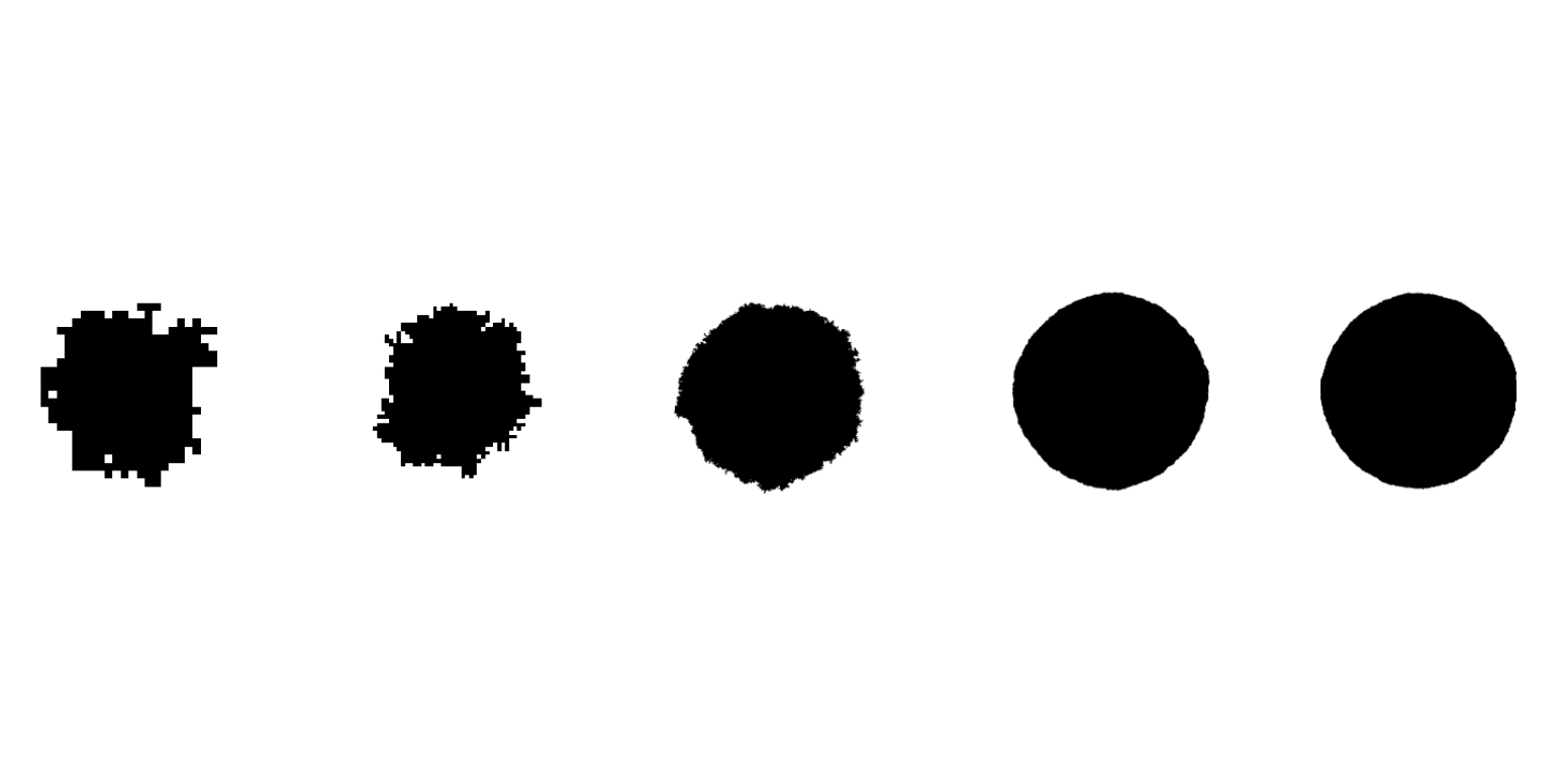
A paradigm in probability is that a little bit of randomness is very random but a whole lot of randomness is not random! Amazing right? This is essentially the contents of the Laws of Large Numbers, and as it turns out, we also have a Law of Large Numbers for FPP! Recall that the definition of the ball of radius time, \(B(t)\) is the set of points that can be reached from the origin by time at most \(t\). What happens if we let \(t\) grow a lot? Well the ball will also grow a lot no shit Sherlock. But what happens if also keep zooming out of the screen at rate \(t\) as time grows? Will be see anything? Will the ball still cover our field of vision? Or conversely, will it shrink into nothingness, i.e: is timescale \(t\) too fast to zoom out? It turns out that it is just about the right one! In fact, due to a beautiful Theorem by Cox and Durret, we know that if the passage times are "nice enough" (just some integrability conditions), then there will exist some set \(\mathcal{B}\) that is convex, symmetric, nonempty, and deterministic (wow!) such that the rescaled ball \(B(t)/t\) (i.e: what we see as we zoom out of the screen) will in fact be Hausdorff-distance at most \(\epsilon\) of \(\mathcal{B}\) almost surely. If you don't know what Hausdorff distance means, just think that if it is very small, then the two objects would look almost like the same picture.
First Passage Percolation (4/4)

This is the last thing I'll say about FPP, and I won't say much about this one because we just don't know much about the damn thing! Suppose that you put two competing species in your graph, and let them explore the graph through the FPP much as like the ball would start to explore the graph, but stop them from "eating each other", so that an interface is created between them when they meet. What can we say about this boundary as we zoom out of the graph? Can we conotrol how much it fluctuates up and down? Can we describe it as a random curve in the scaling limit? We don't know! Similar results are known in related models, but as far as I know, not much is known for this one.